AWS Injector Module– The AWS Injector module easily connects any tag data from the Ignition into the Amazon Web Services (AWS) cloud infrastructure. With a simple configuration, tag data will flow into the AWS KinesisStreams or DynamoDB using an easy to read JSON representation to take full advantage of AWS and all the benefits it offers.
Connects to any Ignition TAG Data
Easy to Configure
For use on the Ignition Gateway or Ignition Edge
Supports Store & Forward
The diagram below shows how using the AWS Injector Module connects OT data into the AWS Web Services. Data is streamed into AWS Kinesis for real-time, streaming or batch analytics.
Azure Injector Module – The AZURE Injector Module easily connects any tag data from Ignition into the Microsoft Azure cloud infrastructure through the IoT Hub. With a simple configuration, tag data will flow into the Azure IoT Hub using an easy to read JSON representation.
Connects to any Ignition TAG Data
Easy to Configure
For use on the Ignition Gateway or Ignition Edge
Supports Store & Forward – Coming Soon!
The diagram below shows how the Cirrus Link Azure Injector Module connects OT data to Microsoft Azure Cloud Services. Operational data is published to the Azure IoT Hub using MQTT and made available to all the Analytic tools Azure has to offer.
Google Cloud Platform Injector Module – The Google Cloud Platform Injector Module enables end users of Ignition to select data from the Ignition platform to be sent into the IBM Cloud infrastructure to utilize their services for analytics. With a simple configuration, tag data will flow into the IBM Cloud giving users easy access to all the tools and big data analysis the platform has to offer
Connects to any Ignition TAG Data
Easy to Configure
For use on the Ignition Gateway or Ignition Edge
Supports Store & Forward – Coming Soon!
The diagram below shows how the Cirrus Link Google Cloud Platform Injector Module connects OT data to their services.
IBM Cloud Injector Module – The IBM Cloud Injector Module end users of Ignition to select data from the Ignition platform to be sent into the IBM Cloud infrastructure to utilize their services for analytics. With a simple configuration, tag data will flow into the IBM Cloud giving users easy access to all the power of IBM Watson’s machine learning and predicative maintenance.
Connects to any Ignition TAG Data
Easy to Configure
For use on the Ignition Gateway or Ignition Edge
Supports Store & Forward – Coming Soon!
The diagram below shows how the Cirrus Link IBM Cloud Injector Module connects OT data to the IBM Cloud Services.
Whether you're shifting ETL workloads to the cloud or visually building data transformation pipelines, version 2 of Azure Data Factory lets you leverage conventional and open source technologies to move, prep and integrate your data.
The second major version of Azure Data Factory, Microsoft's cloud service for ETL (Extract, Transform and Load), data prep and data movement, was released to general availability (GA)about two months ago. Cloud GAs come so fast and furious these days that it's easy to be jaded. But data integration is too important to overlook, and I wanted to examine the product more closely.
Azure Data Factory v2 allows visual construction of data pipelines
Roughly thirteen years after its initial release, SQL Server Integration Services (SSIS) is still Microsoft's on-premises state of the art in ETL. It's old, and it's got tranches of incremental improvements in it that sometimes feel like layers of paint in a rental apartment. But it gets the job done, and reliably so.
In the cloud, meanwhile, Microsoft's first release of Azure Data Factory (ADF) was, to put it charitably, a minimal viable product (MVP) release. Geared mostly to Azure data services and heavily reliant on a JSON-based, handed-coded approach that only a Microsoft Program Manager could love, ADF was hardly a worthy successor to the SSIS legacy.
Clean slate
But ADF v2 is a whole new product:
It's visual (the JSON-encoded assets are still there, but that's largely hidden from the user)
It has broad connectivity across data sources and destinations, of both Microsoft and non-Microsoft pedigrees
It's modern, able to use Hadoop (including MapReduce, Pig and Hive) and Spark to process the data or use its own simple activity construct to copy data
It doesn't cut ties with the past; in fact, it serves as a cloud-based environment for running packages designed in with the on-premises SSIS
The four points above tell the high-level story fairly well, but let's drill down a bit to make those points a bit more concrete.
Connectivity galore
First off, data sources. Microsoft of course supports its own products and services. Whether it's Microsoft's on-premises flagship SQL Server, PC thorn-in-the-side Access, or in-cloud options like Azure SQL Database, SQL Data Warehouse, Cosmos DB, Blob, file and table storage or Data Lake Store (v1 or v2), ADF can connect to it. And while a connector for Excel files is conspicuously absent, saving a CSV file from Excel allows its data to be processed in ADF using the File System connector.
But there's lots more, including Oracle, DB2, Sybase and Postgres in the RDBMS world; Teradata, Greenplum, Vertica and Netezza data warehouse platforms; MongoDB, Cassandra and Couchbase from the NoSQL scene; HDFS, Hive, Impala, HBase, Drill, Presto and Spark from the open source realm; SAP BW and SAP HANA in the BI/analytics world; Dynamics, Salesforce, Marketo, Service Now and Zoho from the SaaS world and even Amazon Redshift, Amazon S3, Amazon Marketplace Web Service and Google BigQuery on the competitive cloud side.
ADF v2 connects to an array of data stores, both from the Microsoft and competitive worlds
The core unit of work in ADF is a pipeline, made up of a visual flow of individual activities. Activities are little building blocks, providing flow and data processing functionality. What's unusual and impressive here is the degree of logical and control of flow capabilities, as well as the blend of conventional technologies (like SSIS packages and stored procedures) and big data technologies (like Apache Hive Jobs, Python Scripts and Databricks notebooks).
A broad range of activities are on offer. Some of the more interesting ones are highlighted here
The pipelines are constructed visually, and even dragging a single activity onto the canvas allows a great deal of work to be done. In the figure at the beginning of this post, you can see that a single activity allows an entire Python script to be executed on Apache Spark, optionally creating the necessary HDInsight cluster on which the script will be run.
DataOps on board
ADF v2 also allows for precise monitoring of both pipelines and the individual activities that make them up, and offers accompanying alerts and metrics (which are managed and rendered elsewhere, in the Azure portal).
And as as good as the visual interface in v2 versus that of v1 is, ADF offers a range of developer interfaces to the service as well. These include Azure Resource Manager templates, a REST API interface, a Python option, and support for both PowerShellscripts and .NET code.
Behind the scenes
There are also elements to ADF v2 "under the covers" that are worth mentioning. For example, ADF v2 doesn't just support disparate data sources, but moves data between them at great scale when it uses its Azure Integration Runtime. (Microsoft says that ADF can move 1 TB of data from Amazon S3 to Azure SQL Data Warehouse in under 15 minutes.) Scale-out management of this facility is handled for the user by ADF itself. It's managed on a per-job basis and completely serverless, from the user's point of view.
ADF v2 also leverages the innate capabilities of the data stores to which it connects, pushing down to them as much of the heavy work as possible. In fact, the Azure Integration Runtime is less of a data transformation engine itself and more of a job orchestrator and data movement service. As you work with the individual activities, you find that much of the transformation work takes place in the data stores' native environments, using the programming languages and constructs they support.
Quo vadis
Compared to other data pipeline products, ADF v2 is both more evolved and less rich. Its innate capabilities are more limited, but its ability to connect, orchestrate, delegate and manage, using a combination of legacy and modern environments, is robust. It will provide Microsoft and Azure customers with an excellent data transformation and movement foundation for some time to come, and its accommodation of SSIS package lift-and-shift to the cloud makes it Enterprise-ready and -relevant right now.
How to add users to groups in Linux; How to remove users from groups
From security reasons, the users and groups are very important in Unix and Linux systems. Every OS geek should know how to create users and groups,add users to groups or modify user and group account information.
In this article, I will teach you how to add users to groups in Linux.
How to create users with custom primary and secondary groups:
I will create the groups and set them as primary and secondary groups for the newly created user:
Creating the groups jim, michael, and johnson:
$ sudo groupadd jim

$ sudo groupadd michael

$ sudo groupadd johnson
Verifying if the groups have been created, and finding out their GIDs:
Creating the test3 user with jim as a primary group and michael and johnson as secondary groups with useradd: the -g parameter is for adding the user to the primary group, and -G for the secondary groups. Only one group can be set as a primary group.
$ sudo useradd -g jim -G michael,johnson test3

$ id test3

uid=1015(test3) gid=1039(jim) groups=1039(jim),1040(michael),1041(johnson)
The GID displayed in the id commands' output is the ID of the primary group.
Creating the test4 user with the same primary and secondary groups as test3, by using the GIDs:
Usermod is used for changing the user account information. The usermod command’s parameters are the same as the useradd parameters: -g for the primary group and -G for secondary groups.
How to remove users from secondary groups:
The gpasswd command is used for working with groups.
How to remove a user from a group with gpasswd: gpasswd -d username groupname.
$ id test4

uid=1016(test4) gid=1039(jim) groups=1039(jim),1040(michael),1041(johnson)

$ sudo gpasswd -d test4 johnson

Removing user test4 from group johnson

$ id test4

uid=1016(test4) gid=1039(jim) groups=1039(jim),1040(michael)
To remove a user’s primary group, set a new group as primary for that user and after that, remove the user from the old primary group. _______________________________________________________________________________________
5 Useradd Command Examples, With Explanations
Now, I will show you 10 more useradd oneliners, for creating users in all the Linux and Unix systems.
-m -d /home/geeks/mike2 : the -m argument creates the /home/geeks/mike2 homedirectory, specified by the -d argument . as you can notice, the homedir can be different that /home/user_name
-s /bin/zsh : the -s is used for specifing the user’s default shell, /bin/zsh in the case
-c “the mike2 user” : extra information about the user
-u 1099 : the new user’s UID, in this case 1099
-g 1050 : the user belongs to the group with the 1050 GID
-m -d /home/mike3 : the -m argument creates the /home/mike3 homedirectory, specified by the -d argument
-s /usr/sbin/nologin : the -s is used for specifing the user’s default shell, in this case /usr/sbin/nologin . mike3 cannot login to the system with su, but can login by ssh. Read more about the nologin shells here.
-c “nologin user” : extra information about the user
-M : the -M argument tells the system not to create a home directory
-N : the -N argument tells the system not to create a group having the user’s name
-r : the -r arguments is for creating a system user
-s /bin/false : the -s is used for specifing the user’s default shell, /bin/false in this case. The users having /bin/false as the default shell, cannot login to the system. Read more about the nologin shells here.
-c “system user” : extra information about the user
BigQuery just announced the ability to cluster tables — which I’ll describe here. If you are looking for massive savings in costs and querying times, this post is for you.
Warning: This post plays with several terabytes of data. Set up your BigQuery cost controls, buckle up, keep calm, and query on.
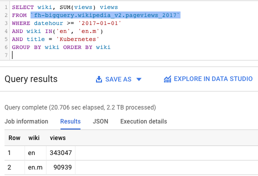
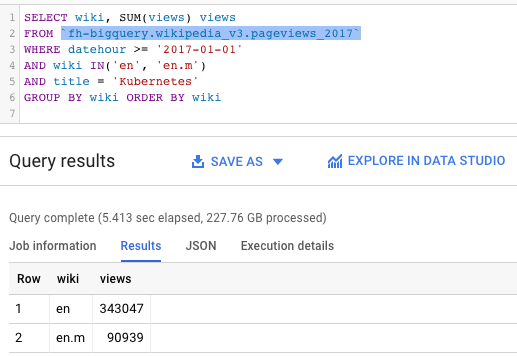
Can you spot the huge difference between the query on the left and the one on the right?
Same query over almost the same tables — one is clustered, the other is not. Faster and more efficient.
What can we see here:
Kubernetes was a popular topic during 2017 in Wikipedia — with more than 400,000 views among the English Wikipedia sites.
Kubernetes gets way less pageviews on the mobile Wikipedia site than on the traditional desktop one (90k vs 343k).
But what’s really interesting:
The query on the left was able to process 2.2 TB in 20 seconds. Impressive, but costly.
The query on the right went over a similar table — but it got the results in only 5.4 seconds, and for one tenth of the cost (227 GB).
What’s the secret?
Clustered tables!
Now you can tell BigQuery to store your data “sorted” by certain fields — and when your queries filter over these fields, BigQuery will be smart enough to only open the matching clusters. In other words, you’ll get faster and cheaper results.
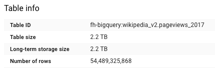
Previously I explained my lazy loading of Wikipedia views into partitioned yearly BigQuery tables. As a reminder, just for 2017 we will be querying more than 190 billion of pageviews, over 3,927 Wikipedia sites, covered by over 54 billion rows (2.2 TBs of data per year).
To move my existing data into a newly clustered table I can use some DDL:
CREATE TABLE `fh-bigquery.wikipedia_v3.pageviews_2017`
PARTITION BY DATE(datehour)
CLUSTER BY wiki, title
OPTIONS(
   description="Wikipedia pageviews - partitioned by day, clustered by (wiki, title). Contact https://twitter.com/felipehoffa"
   , require_partition_filter=true
)
AS SELECT * FROM `fh-bigquery.wikipedia_v2.pageviews_2017`
WHERE datehour > '1990-01-01' # nag
-- 4724.8s elapsed, 2.20 TB processed
Note these options:
CLUSTER BY wiki, title: Whenever people query using the wiki column, BigQuery will optimize these queries. These queries will be optimized even further if the user also filters by title. If the user only filters by title, clustering won’t work, as the order is important (think boxes inside boxes).
require_partition_filter=true: This option reminds my users to always add a date filtering clause to their queries. That’s how I remind them that their queries could be cheaper if they only query through a fraction of the year.
4724.8s elapsed, 2.20 TB processed: It took a while to re-materialize and cluster 2.2 TB of data — but the future savings in querying makes up for it. Note that you could run the same operation for free with a bq export/load combination — but I like the flexibility that DDL supports. Within theSELECT * FROM I could have filtered and transformed my data, or added more columns just for clustering purposes.
Better clustered: Let’s test some queries
SELECT * LIMIT 1
SELECT * LIMIT 1 is a known BigQuery anti-pattern. You get charged for a full table scan, while you could have received the same results for free with a table preview. Let’s try it on our v2 table:
SELECT *
FROM `fh-bigquery.wikipedia_v2.pageviews_2017`
WHERE DATE(datehour) BETWEEN '2017-06-01' AND '2017-06-30'
LIMIT 1
1.7s elapsed, 180 GB processed
Ouch. 180 GB processed — but at least the date partitioning to cover only June worked. But the same in v3, our clustered table:
SELECT *
FROM `fh-bigquery.wikipedia_v3.pageviews_2017`
WHERE DATE(datehour) BETWEEN '2017-06-01' AND '2017-06-30'
LIMIT 1
1.8s elapsed, 112 MB processed
Yes!!! With a clustered table we can now do a SELECT * LIMIT 1, and it only scanned 0.06% of the data (in this case).
Base query: Barcelona, English, 180->10GB
SELECT wiki, SUM(views) views
FROM `fh-bigquery.wikipedia_v2.pageviews_2017`
WHERE DATE(datehour) BETWEEN '2017-06-01' AND '2017-06-30'
AND wiki LIKE 'en'
AND title = 'Barcelona'
GROUP BY wiki ORDER BY wiki
18.1s elapsed, 180 GB processed
Any query similar to this will incur costs of 180 GB on our v2 table. Meanwhile in v3:
SELECT wiki, SUM(views) views
FROM `fh-bigquery.wikipedia_v3.pageviews_2017`
WHERE DATE(datehour) BETWEEN '2017-06-01' AND '2017-06-30'
AND wiki LIKE 'en'
AND title = 'Barcelona'
GROUP BY wiki ORDER BY wiki
3.5s elapsed, 10.3 GB processed
On a clustered table we get the results on 1/6th of the time, for 5% of the costs.
Don’t forget the clusters order
SELECT wiki, SUM(views) views
FROM `fh-bigquery.wikipedia_v3.pageviews_2017`
WHERE DATE(datehour) BETWEEN '2017-06-01' AND '2017-06-30'
-- AND wiki = 'en'
AND title = 'Barcelona'
GROUP BY wiki ORDER BY wiki
3.7s elapsed, 114 GB processed
If I don’t make use of my of my clustering strategy (in this case: filtering by which of the multiples wikis first), then I won’t get all the possible efficiencies — but it’s still better than before.
Smaller clusters, less data
The English Wikipedia has way more data than the Albanian one. Check how the query behaves when we look only at that one:
SELECT wiki, SUM(views) views
FROM `fh-bigquery.wikipedia_v3.pageviews_2017`
WHERE DATE(datehour) BETWEEN '2017-06-01' AND '2017-06-30'
AND wiki = 'sq'
AND title = 'Barcelona'
GROUP BY wiki ORDER BY wiki
2.6s elapsed, 3.83 GB
Clusters can LIKE and REGEX
Let’s query for all the wikis that start with r, and for the titles that match Bar.*na:
SELECT wiki, SUM(views) views
FROM `fh-bigquery.wikipedia_v3.pageviews_2017`
WHERE DATE(datehour) BETWEEN '2017-06-01' AND '2017-06-30'
AND wiki LIKE 'r%'
AND REGEXP_CONTAINS(title, '^Bar.*na')
GROUP BY wiki ORDER BY wiki
4.8s elapsed, 14.3 GB processed
That’s nice behavior —clusters can work with LIKE and REGEX expressions, but only when looking for prefixes.
If I look for suffixes instead:
SELECT wiki, SUM(views) views
FROM `fh-bigquery.wikipedia_v3.pageviews_2017`
WHERE DATE(datehour) BETWEEN '2017-06-01' AND '2017-06-30'
AND wiki LIKE '%m'
AND REGEXP_CONTAINS(title, '.*celona')
GROUP BY wiki ORDER BY wiki
(5.1s elapsed, 180 GB processed
That takes us back to 180 GB — this query is not using clusters at all.
JOINs and GROUP BYs
This query will scan all data within the time range, regardless of what table I use:
SELECT wiki, title, SUM(views) views
FROM `fh-bigquery.wikipedia_v2.pageviews_2017`
WHERE DATE(datehour) BETWEEN '2017-06-01' AND '2017-06-30'
GROUP BY wiki, title
ORDER BY views DESC
LIMIT 10
64.8s elapsed, 180 GB processed
That’s a pretty impressive query — we are grouping thru 185 million combinations of (wiki, title) and picking the top 10. Not a simple task for most databases, but here it looks like it was. Can clustered tables improve on this?
SELECT wiki, title, SUM(views) views
FROM `fh-bigquery.wikipedia_v3.pageviews_2017`
WHERE DATE(datehour) BETWEEN '2017-06-01' AND '2017-06-30'
GROUP BY wiki, title
ORDER BY views DESC
LIMIT 10
22.1 elapsed, 180 GB processed
As you can see here, with v3 the query took one third of the time: As the data is clustered, way less shuffling is needed to group all combinations before ranking them.
FAQ
My data can’t be date partitioned, how do I use clustering?
Two alternatives: 1. Use ingestion time partitioned table with clustering on the fields of your interest. This is the preferred mechanism if you have > ~10GB of data per day. 2. If you have smaller amounts of data per day, use a column partitioned table with clustering, partitioned on a “fake” date optional column. Just use the value NULL for it (or leave it unspecified, and BigQuery will assume it is NULL). Specify the clustering columns of interest.
Engineers tip: I’ve heard that for now it’s better if you load data into your clustered tables once per day. On that tip, I’ll keep loading the hourly updates to v2, and insert the results into v3 once the day is over. From the docs: “Over time, as more and more operations modify a table, the degree to which the data is sorted begins to weaken, and the table becomes partially sorted”.
Next steps
Clustered tables in only one of many new BigQuery capabilities: Check out GIS support (geographical), and BQML capabilities (machine learning within BigQuery).
 AWS Injector Module – The AWS Injector module easily connects any tag data from the Ignition into the Amazon Web Services (AWS) cloud infrastructure. With a simple configuration, tag data will flow into the AWS Kinesis Streams or DynamoDB using an easy to read JSON representation to take full advantage of AWS and all the benefits it offers.


 Google Cloud Platform Injector Module – The Google Cloud Platform Injector Module enables end users of Ignition to select data from the Ignition platform to be sent into the IBM Cloud infrastructure to utilize their services for analytics. With a simple configuration, tag data will flow into the IBM Cloud giving users easy access to all the tools and big data analysis the platform has to offer
 IBM Cloud Injector Module – The IBM Cloud Injector Module end users of Ignition to select data from the Ignition platform to be sent into the IBM Cloud infrastructure to utilize their services for analytics. With a simple configuration, tag data will flow into the IBM Cloud giving users easy access to all the power of IBM Watson’s machine learning and predicative maintenance.