Thursday, 11 October 2018

Hive useful commands

Regularly used common commands:
DESCRIPTION
COMMAND
Autocomplete
hive> Press Tab key
Display all 436 possibilities? (y or n)If you enter y, you’ll get a long list of all the keywords
Navigation Keystrokes
Use the up arrow and down arrow keys to scroll through previous commandsCtrl+A goes to the beginning of the lineCtrl+E goes to the end of the lineDelete key will delete the character to the left of the cursor
Command History
Hive saves the last 100,00 lines into a file $HOME/.hivehistory
Shell Execution
type ! followed by the command and terminate the line with a semicolon (;)
hive> ! /bin/echo “Hello World”;
Hello World
hive> ! pwd;/home/me/hiveplay
(Note: Don’t invoke interactive commands that require user input. Shell “pipes” don’t work and neither do file “globs.”For example, ! ls *.hql; will look for a file named *.hql;, rather than all files that end with the .hql extension.)
To Print Current DB in use
set hive.cli.print.current.db=true; (or)
set hiveconf:hive.cli.print.current.db=true;
To remove current db name display in hive shell
set hiveconf:hive.cli.print.current.db=false;
Specifying Metastore location for each user
set hive.metastore.warehouse.dir=/user/myname/hive/warehouse;
system Namespace (provides read-write access to Java system properties)
set system:user.name; (or)
set system:user.name=yourusername;
env Namespace (provides read-only access to environment variables)
set env:HOME;
Hadoop dfs commands inside Hive shell
Exclude hadoop keyword and end the command with semicolon(;) as below:
hive> dfs -ls / ;
(Note: This method of accessing hadoop commands is actually more efficient than using the hadoop dfs … equivalent at the bash shell, because the latter starts up a new JVM instance each time, whereas Hive just runs the same code in its current process.)
Execute hive queries from a .hqlfile
source /unix-path/to/file/withqueries.hql;
Print Column Headers
set hive.cli.print.header=true;
Show complete details of a table
SHOW CREATE TABLE mytable; (or)
DESCRIBE [FORMATTED] [db_name.]table_name[.complex_col_name …] (or)
DESCRIBE EXTENDED mytable;
hive> SHOW CREATE TABLE employees;
OK
CREATE TABLE `employees`(
  `emplid` string COMMENT 'from deserializer',
  `name` string COMMENT 'from deserializer',
  `age` string COMMENT 'from deserializer',
  `salary` string COMMENT 'from deserializer',
  `dept` string COMMENT 'from deserializer')
ROW FORMAT SERDE
  'org.apache.hadoop.hive.contrib.serde2.RegexSerDe'
WITH SERDEPROPERTIES (
  'input.regex'='(.{4})(.{35})(.{3})(.{11})(.{4})')
STORED AS INPUTFORMAT
  'org.apache.hadoop.mapred.TextInputFormat'
OUTPUTFORMAT
  'org.apache.hadoop.hive.ql.io.HiveIgnoreKeyTextOutputFormat'
LOCATION
  'hdfs://sandbox.hortonworks.com:8020/user/hue/tmp/fixed_employees'
TBLPROPERTIES (
  'COLUMN_STATS_ACCURATE'='true',
  'numFiles'='0',
  'totalSize'='0',
  'transient_lastDdlTime'='1455035524')
Time taken: 3.399 seconds, Fetched: 21 row(s)
Get columns names of the table
SHOW COLUMNS FROM mytable;
Load data from a local file to the hive table
LOAD DATA LOCAL INPATH ‘/unix-path/myfile’ INTO TABLE mytable;
Load data from hdfs file to the hive table
LOAD DATA INPATH ‘/hdfs-path/myfile’ INTO TABLE mytable;
Data Types
Numeric Data Types:
>> TINYINT (1-byte signed integer, from -128 to 127)
>> SMALLINT (2-byte signed integer, from -32,768 to 32,767)
>> INT (4-byte signed integer, from -2,147,483,648 to 2,147,483,647)
>> BIGINT (8-byte signed integer, from -9,223,372,036,854,775,808 to 9,223,372,036,854,775,807)
>> FLOAT (4-byte single precision floating point number)
>> DOUBLE (8-byte double precision floating point number)
>> DECIMAL (or) DECIMAL(precision, scale)
(Precision of 38 digits. User definable precision and scale)
Date/Time Types:
>> TIMESTAMP (UTC time. Format ‘YYYY-MM-DD HH:MM:SS.fffffffff’ (9 decimal place precision)
Ex: ‘2012-02-03 12:34:56.123456789’
>> DATE (Format: ‘YYYY- MM- DD’ The range of values supported for the Date type is be 0000- 01- 01
to 9999- 12- 31, dependent on support by the primitive Java Date type.)
String Types:
>> STRING
>> VARCHAR (Length specifier between 1 and 65355)
>> CHAR (Fixed-length. The maximum length is fixed at 255)
Misc Types:
>> BOOLEAN
>> BINARY
Complex Types:
>> arrays: ARRAY
>> maps: MAP
>> structs: STRUCT
>> union: UNIONTYPE
Dynamic Partition
Given below are the configuration properties for dynamic partition inserts. Note by default 
dynamic partition inserts are disabled.
CONFIGURATION PROPERTY
DEFAULT
NOTE
hive.exec.dynamic.partition
false
Needs to be set to true to enable dynamic partition inserts
hive.exec.dynamic.partition.mode
strict
In strict mode, the user must specify at least one static partition in case the user accidentally overwrites all partitions, in nonstrict mode all partitions are allowed to be dynamic
hive.exec.max.dynamic.partitions.pernode
100
Maximum number of dynamic partitions allowed to be created in each mapper/reducer node
hive.exec.max.dynamic.partitions
1000
Maximum number of dynamic partitions allowed to be created in total
hive.exec.max.created.files
100000
Maximum number of HDFS files created by all mappers/reducers in a MapReduce job
hive.error.on.empty.partition
false
Whether to throw an exception if dynamic partition insert generates empty results
Hive One Shot commands
DESCRIPTION
COMMAND
To Print Current DB in use
$ hive –hiveconf hive.cli.print.current.db=true
Specify a file of commands for the CLI to run as it starts, before showing you the prompt
$ cat hiveproperties.txt
set hive.cli.print.current.db=true;
set system:user.name;
$ hive -i hiveproperties.txt
system:user.name=yourusername
hive>
Adding the -e execute Hive queries
$ hive -e “SELECT * FROM mytable LIMIT 3”;
Adding the -S for silent mode removes the OK and Time taken … lines, as well as other inessential output
$ hive -S -e “SELECT * FROM mytable LIMIT 3”
Useful trick for finding a property name that you can’t quite remember
$ hive -S -e “set” | grep warehouse_or_pattern

Comments in Hive scripts starts with double hyphen (‐‐) followed by space and then comment description.
Hive scripts have the extension .hql
$ cat hivescript.hql
‐‐ Comment line1
‐‐ Comment line2
SELECT * FROM mytable LIMIT 3;
Executing Hive Queries from .hql files
$ hive -f /unix-path/to/file/hivescript.hql
Hive variables (The env namespace is useful as an alternative way to pass variable definitions to Hive)
$ YEAR=2012 hive -e “SELECT * FROM mytable WHERE year = ${env:YEAR}”;

5 Tips for efficient Hive queries with Hive Query Language

5 Tips for efficient Hive queries with Hive Query Language


hive query example


Hive on Hadoop makes data processing so straightforward and scalable that we can easily forget to optimize our Hive queries. Well designed tables and queries can greatly improve your query speed and reduce processing cost. This article includes five tips, which are valuable for ad-hoc queries, to save time, as much as for regular ETL (Extract, Transform, Load) workloads, to save money. The three areas in which we can optimize our Hive utilization are:
  • Data Layout (Partitions and Buckets)
  • Data Sampling (Bucket and Block sampling)
  • Data Processing (Bucket Map Join and Parallel execution)
We will discuss these areas in detail below. Also watch our webinar on the topic given by Ashish Thusoo, co-founder of Apache Hive, and Sadiq Sid Shaik, Director of Product at Qubole. Based on the data set we use, Qubole can improve your data set, as illustrated in the example below.
The data consists of three tables. The table Airline Bookings All contains 276 million records of complete air travel trips from an origin to a destination with an itinerary identifier as key. The second table Airline Bookings Origin Only contains the data for the first leg of an itinerary only and also has the itinerary’s identifier as a key. The last table is ‘Census’ containing population information for each US state.
airline-booking
This example data set demonstrates Hive query language optimization.
Tip 1: Partitioning Hive Tables Hive is a powerful tool to perform queries on large data sets and it is particularly good at queries that require full table scans. Yet many queries run on Hive have filtering where clauses limiting the data to be retrieved and processed, e.g. SELECT * WHERE state=’CA’. Hive users tend to have or develop a domain knowledge, understand the data they work with and the queries commonly executed or scheduled. With this knowledge we can identify common data structures that surface in queries. This enables us to identify columns with a (relatively) low cardinality like geographies or dates and high relevance to key queries.
For example, common approaches to slice the airline data may be by origin state for reporting purposes. We can utilize this knowledge to organise our data by this information and tell Hive about it. Hive can utilize this knowledge to exclude data from queries before even reading it. Hive tables are linked to directories on HDFS or S3 with files in them interpreted by the meta data stored with Hive. Without partitioning Hive reads all the data in the directory and applies the query filters on it. This is slow and expensive since all data has to be read. In our example a common reports and queries might be generated on an origin state basis.
This enables us to define at creation time of the table the state column to be a partition. Consequently, when we write data to the table the data will be written in sub-directories named by state (abbreviations). Subsequently, queries filtering by origin state, e.g. SELECT * FROM Airline_Bookings_All WHERE origin_state = ‘CA’, allow Hive to skip all but the relevant sub-directories and data files. This can lead to tremendous reduction in data required to read and filter in the initial map stage. This reduces the number of mappers, IO operations, and time to answer the query.
patritioned
Example Hive table partitioning It is important to consider the cardinality of a potential partition column and avoid fragmenting the data too much. Itinerary ID would be a very poor choice for partitioning. Queries for single itineraries by ID would be very fast but any other query would require to parse a huge amount of directories and files incurring serious overheads.
Additionally, HDFS uses a very large block size of usually 64 MB or more which means that each file, even with only a few bytes of data, will have to allocate that block size on HDFS. This can potentially fill the file system up with large number of files carrying barely any actual data.
Tip 2: Bucketing Hive Tables Itinerary ID is unsuitable for partitioning as we learned but it is used frequently for join operations. We can optimize joins by bucketing ‘similar’ IDs so Hive can minimise the processing steps, and reduce the data needed to parse and compare for join operations. Itinerary IDs, of course, have no real similarity and we only need to achieve that the same itinerary IDs from two tables end up in the same processing bucket.
A simple trick to do this is to hash the data and store it by hash results, which is what bucketing does.
31
Example Hive query table bucketing Bucketing requires us to tell Hive at table creation time by which column to cluster by and into how many buckets. We also have to ensure the bucketing flag is set (SET hive.enforce.bucketing=true;) every time before we write data to the bucketed table.
Importantly, the corresponding tables we want to join on have to be set up in the same manner with the joining columns bucketed and the bucket sizes being multiples of each other to work. The second part is the optimized query for which we have to set a flag to hint to Hive that we want to take advantage of the bucketing in the join (SET hive.optimize.bucketmapjoin=true;).
The SELECT statement then can include a MAPJOIN statement to ensure that the join operation is executed at the map stage by combining only the few relevant files in each mapper task in a distributed fashion from the two tables instead of parsing the full tables.   Example Hive MAPJOIN with bucketing
bucketmap
Tip 3: Bucket Sampling Once our tables are setup with these buckets we can address another important use-case. We often want to query large table joins for a sample. We may want to try out complex queries or explore the data, and we want to do this iteratively, swiftly, and not process the whole data set.
This is particularly difficult because of the joining of the tables since only very little data may overlap on independent samples from two tables. Ideally we would want to sample the relevant data on both tables and join it, i.e. ensure that we sample the same itinerary IDs from both tables and not sets with no or little overlap.
The bucketing on the join column enables us to join specific buckets from two tables with data overlapping on the join column. Effectively, we execute exactly one part of the complete join operation and only incur the cost of it. The hashing function on the ID has the additional benefit of a (somewhat) random nature providing a representative sample.
table-sample
Example Hive TABLESAMPLE on bucketed tables
Tip 4: Block Sampling Similarly, to the previous tip, we often want to sample data from only one table to explore queries and data. In these cases we may not want to go through bucketing the table or we have the need to sample the data more randomly (independent from the hashing of a bucketing column) or at decreasing granularity.
Block sampling provides a powerful syntax to define various ways of sampling the data in a table with the TABLESAMPLE statement. We can use it to sample a certain percentage, number of bytes, or rows of the data. We can use the sampling to approximate information like average distance between origin and destination of our itineraries.
A query using 1% of the data using TABLESAMPLE(1 PERCENT) on a large table will give us a near perfect answer and use up to only a hundredth of the resource and return the result one to two magnitudes faster. In exploratory work or for metrics this approach can be extremely efficient and effective alternative to processing all of the data. The beauty of this solution is that we can scale the sample size with our data size. If we were to explore at Tera- or Petabytes of data we could sample a fraction of percent and get the same actionable information in minutes or less which would otherwise take hours to receive.
Tip 5: Parallel Execution Hadoop can execute map reduce jobs in parallel and several queries executed on Hive make automatically use of this parallelism. However, single, complex Hive queries commonly are translated to a number of map reduce jobs that are executed by default sequentially. Often though some of a query’s map reduce stages are not interdependent and could be executed in parallel.
They then can take advantage of spare capacity on a cluster and improve cluster utilization while at the same time reduce the overall query executions time. The configuration in Hive to change this behaviour is a merely switching a single flag SET hive.exce.parallel=true;.
parallal
Example of Hive parallel stage execution of a query In our example in the image above we can see that the two sub-queries are independent and when we enable parallel execution are processed at the same time.
In our example this reduced the execution time by 50%! Conclusion The five presented tips in this article can easily be applied by anyone using Hive to improve processing and query speed and reduce resource consumption.

Tuesday, 9 October 2018

Getting started with Google BigQuery by Kiran Vasadi


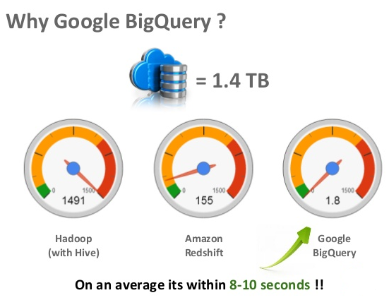
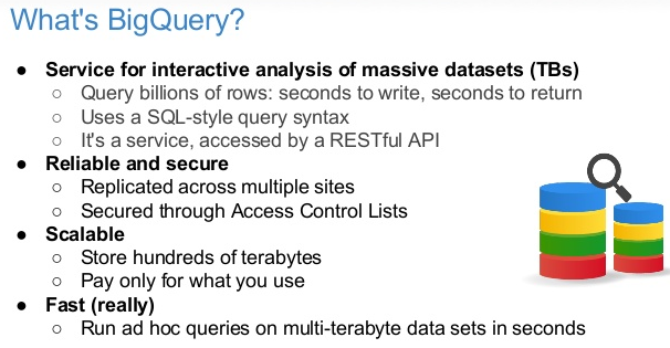
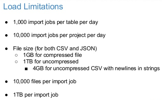
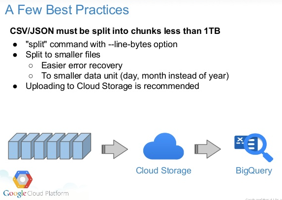
  • Fully Managed structured data store queryable with SQL
  • very easy to use
  • Fast, in that almost no slowdown with BigData
  • Cost-effective
  • Built on Google's infrastructure Components
  • Basic Operations are available within WebUI
  • You can 'dryrun' from Web UI to check the amount of data to be scanned
  • You can use the command line interface (bq) to integrate BigQuery into your workflow
  • API are provided for Python Java


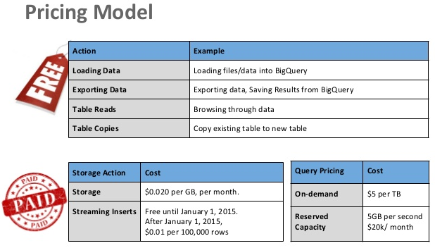
What you pay for


  • Storage - $0.020 per GB / month
  • Queries - $5 per TB processed (scanned)
  • Streaming inserts - $0.01 per 100,000 rows until July 20.2015. After July 20,2015 $0.01 per 200MB, with individual rows calculated using a 1 KB minimum size

A Simple Example

       Load 1TB data to a table every day, keep each table for a month
    
      Query the daily data 5 times every day to aggregation 

      For storage:

      1TB * 20 (tables) = $0.020 * 1000 * 30 = $600

      For Queries:

      1TB * 5 (Queries) * 30(days) = $750


How your data is stored

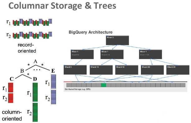
  • Your data is stored
           1. in thousands of disk (depending on the size)

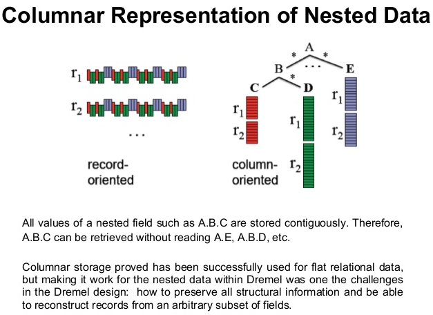
           2. in columnar format

           3. Compressed
               (However, the cost is based on uncompressed size)


  • Record: A Collection of one or more other fields


Regards,
Kiran Kumar Vasadi
Architect Big Data Cloud
Mobile: +918977081119
Skype ID : kiranvasadi

Google Cloud Certified Professional Data Engineer


I am thankful to all those who said No to me It's because of them i did it myself !  ..Einstein